U gebruikt een verouderde browser. Wij raden u aan een upgrade van uw browser uit te voeren naar de meest recente versie.

Fox Rabbit Math Model                                                                               < Previous page       Next page >

Artificial Life: Differential Equations

You can freely download the Fox Rabbit Math Model program. Before you do, first read the copyright statement.

See also:

Computer Simulation:
Fox Hare Field Model

Real life (1):
Lynxes and Snow Hare

Real life (2):
Global Climate Change

Real life (3):
The Covid-19 Pandemic

Introduction: Cyclic behavior

What will happen when there is a system (like a natural habitat, a human community, an economic system, or the entire natural & human world), in which some cause (let's call it 'A') influences this system in such a way that a rise in A causes an effect on another aspect of the system (let's call that one 'B')?

The answer depends on the effect that B, in its turn, will have on A. If an increase in B will cause A to rise even further, you have an example of positive feedback. Systems like these will tend to get out of hand quickly and creata disaster. Positive feedback causes instability. This principle is illustrated with another computer program on this site, PopSim, in the Positive feedback scenario.

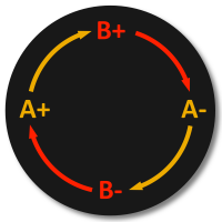
In other systems, situations occur in which some A and B work against each other: when a ris in A makes B rise too, the rise in B will cause A to diminish, like the illustration on the right. This leads to negative feedback, illustrated by PopSim's Negative feedback scenario.

In such systems, a cyclic behavior may appear, exhibiting a stationary kind of stability. Generally speaking: negative feedback causes stability. Systems with this behavior have been studied intensively, both in theoretical models and in real life. Their significance towards the science of sustainability is enormous.

Roorda investigated these systems with the aid of two theoretical models, the two Fox Rabbit computer programs, one of which is described on the current page. For the other model, and for three real-life cases, you see the links at the top of this page.

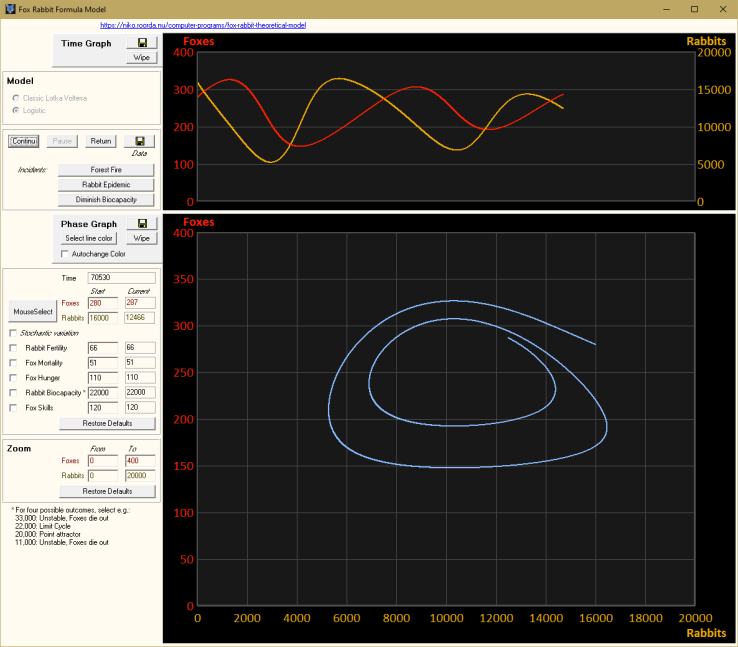
The program shown on this page is a simulation of the growth and decay of two species in a fixed landscape. The species involved are a a prey (symbolically called the  Rabbit ) and its preditor (the  Fox ). In the image on the right, the rabbits represent 'A' while the foxes are 'B'.

(See also: the Introduction to Cyclic Pandemic Behavior.)

About simulations, models and scenarios

Source: The text in this section was published in Chapter 6 of: N. Roorda: Fundamentals of Sustainable Development (English, 3rd edition, 2020); the text is also available in Dutch in Basisboek Duurzame Ontwikkeling (4th edition, 2020) and in German in Grundlagen der nachhaftigen Entwicklung (Springer Vieweg, 2021). Several exercises that are accessories to these books apply the two Fox Rabbit computer programs.


One could call it ‘experimental futurology’, given that it envisions the future in such a way that it can be experimented with. In reality, we are not dealing with the future here, but rather with one possible future. The process involves using a computer and specially designed applications that are called simulation software.

The word simulation literally refers to ‘imitation’ and it involves mimicking the real world, or a part thereof, on a computer. Some of this software was designed as a game, with the Sims and SimCity amongst the best known of these. Both those names come from the word ‘simulation’. Other simulation packages are intended for more serious purposes, being used to see what the weather will be in the near future, for example, for the weather forecasts that we see and read. A simulation program uses a model, which is a simplified representation of reality. Simulation software is not the only type of model – a plastic kit of an airplane is also a model, just like a map in an atlas is a model of a real country. A photograph serves as a model of the subject pictured, and a series of formulas that collectively detail the orbits of the planets is a model of a planetary system.

The word ‘simplified’ in the definition of ‘model’ is very important, as every model, be it a toy airplane, a SimCity landscape or a representation of the atmosphere in weather software, is derived from the actual situation by simplifying many of the real aspects. This is inevitable, as a model of the universe that is not simplified in any sense would simply be the universe itself. Reality is simplified through the following:

  • shrinking the scale
  • omitting surrounding areas
  • omitting some of the components
  • simplifying other components
  • a two-dimensional representation of a three-dimensional scenario (e.g. on a computer monitor)
  • simplifying events, the underlying natural laws or the economic or judicial laws

A common error people commit when using models – especially simulation software – is that they forget about the simplifications and draw conclusions about the real world from the simulation results without exercising any caution whatsoever.

The choice of model is the first step when performing a simulation, with the second step involving the selection of a scenario. A scenario is the plan for the events that are set to take place in the simulation. The word originally referred to plays – and later, films – to outline the scenes that made up the story, wherein a scenario required that every scene was written out in advance. This is not required for a computer simulation, where the only thing necessary is that the starting situation is determined. The computer then calculates, with the aid of the model, the step-by-step progress of events from that starting point onwards. This is how the future is ‘calculated’.

An example demonstrates this. The example is often labelled as the ‘prey-predator model’. This model examines the progress of two types of animal – predators and prey, such as foxes and rabbits. The model is instructive as, instead of foxes and rabbits, it could just as well deal with people and their consumption of food and other resources. This allows investigating the consequences of overexploitation.

In its simplest form the model consists of just two mathematical formulas. One of them deals with the increase in the fox population when they eat rabbits, and with its decrease when the foxes die of old-age. The other formula deals with the decrease in the rabbit population when they are eaten by foxes, and with its increase through reproduction.

This model is extremely simplified. The genders of the foxes and rabbits don’t play a role, nor do the landscape and the grass growth, the change of seasons or the emigration and immigration of the foxes and rabbits to or from other areas. Another thing not included in this model is the role played by chance. Because the chance factor is absent, the future becomes wholly predictable, and once the starting situation is determined – being the starting population of the rabbits and the foxes – the scenario becomes established.  Once the computer starts working with this model, it returns a neat and regular graph like the one [on top of this webpage]. Repeat the simulation using the same scenario and the exact same graph will be reproduced.

End of citation from Fundamentals of Sustainable Development.


Two Models

The program Fox Rabbit Math Model applies two different models in order to calculate the processes. Each of them consists of a set of mathematical formulae which are differential equations.

The Lotka-Volterra Model

Sources:
    Lotka, A. J. (1925): Elements of physical biology. Williams & Wilkins Co, Baltimore'
    Volterra, V. (1926): Variazioni e fluttuazioni del numero d'individui in specie animali conviventi. Williams & Wilkins Co, Baltimore.

One of the oldest, and certainly the most popular models was developed by Lotka and Volterra. They formulated the following set of linked differential equations:

With:  R =
F =
r =
a =
E =
c =

number of Rabbits
number of Foxes
natural growth rate of rabbits  (a constant)
catch skills of foxes  (a constant)
efficiency of fox reproduction (no. of rabbits needed for 1 newborn fox)  (a constant)
natural mortality rate of foxes  (a constant)

The two formulae can be understood as follows:

  • The growth rate of the rabbit population (dR/dt) is directly proportional to the existing number of rabbits, hence:  r.R.
  • The decrease of the number of rabbits is due to the number of them that is caught by the foxes, and is directly proportional to both the number of rabbits (the more rabbits exist, the more likely that one of them is caught) and the number of foxes (the more foxes exist, the more likely it is that one of them catches a rabbit), hence:  - a.FR.
  • The growth rate of the fox population (dF/dt) is directly proportional to the number of rabbits they eat, hence:  E.a.FR.
  • Finally, the decrease of the fox number is due to natural death, and is proportional to the number of foxes, hence:  - m.F.

This explanation makes clear that the Lotka-Volterra model indeed is a severe simplification of reality. Nevertheless, the model shows some interesting characteristics that show a remarkable resemblance with real life in various contexts. The model has been used with a certain level of success, not only in biology & ecology, but also in economy and in historical science, e.g. describing human population development.

When appropriate values for the constants and for the numbers of animals at the starting time (t = 0) are chosen, a cyclic process appears in which the numbers of rabbits go up, followed by the number of foxes. Due to the increase in fox number, the rabbit population starts shrinking, causing the fox population to do the same, which in its turn allows the rabbit numbers to go up again, etc. As a result, the computer program delivers a coupled set of waves:

This cyclic process is stationary: again and again, the exact same trajectory is followed. With other choices of the initial numbers, larger or smaller curves are created. A 'phase diagram' - in which the rabbit numbers are depicted on the horizontal axis and the fox numbers on th vertical one - shows this even more clearly. Below, three such cycles are shown, each starting from a different initial state. In this diagram, the three cycles move counterclockwise.

A Logistic Model

Sources:
    Kuznetsov, Y.A., S. Muratori & S. Rinaldi (1992): Bifurcations and chaos in a periodic predator–prey model. International Journal of Bifurcation and Chaos 1992;2(1):117–128. http://dx.doi.org/10.1142/S0218127492000112.
    Wang, W. & J.H. Sun (2003): On the predator–prey system with Holling(n+1) functional response. Acta Mathematica Sinica. 2003;23(1):1–6.
http://dx.doi.org/10.1007/s10114-005-0603-8.
    Hoff, Quay van der, Johanna C. Greeff & P. Hendrik Kloppers (2013): Numerical investigation into the existence of limit cycles in two-dimensional predator–prey systems. South African Journal of Science, Volume 109 | Number 5/6, May/June 2013, on ResearchGate.

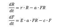
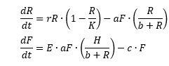
An eternally repeating process does not show much similarity with the real world. 'History never repeats itself', as a saying goes. So, several alternative models have been developed that do exhibit change. One of them, ' Logistic Model', is applied in the Fox Rabbit Math Model' computer program. It is an expansion of the Lotka-Volterra Model.

In this model, two new constant are added, as the differential equations show:

With:  K =
b =

biocapacity available to the rabbits  (a constant)
'half saturation constant', i.e. the number of prey at which the predation rate is half maximum.

Due to the limiting role of the biocapacity K, i.e. the maximum 'healthy' number of rabbits, the system has an upper boundary, which prevents the rabbits from growing indefinitely. Hence, the growth is not unlimited but logistic. You can read more about that at the page of another computer program by Roorda: PopSim, in the section Four basic growth scenarios, specifically in graph B: inhibited growth.

In this case, there is a major difference with the well-known principle of inhibited growth towards a maximum which is determined by the biocapacity. Such growth usually ends in a static world, in which the system is 'frozen'. Here, however, the system ends in a dynamic equilibrium, which develops through a series of cycles towards a stationary state called a limit cycle. The image illustrates this.

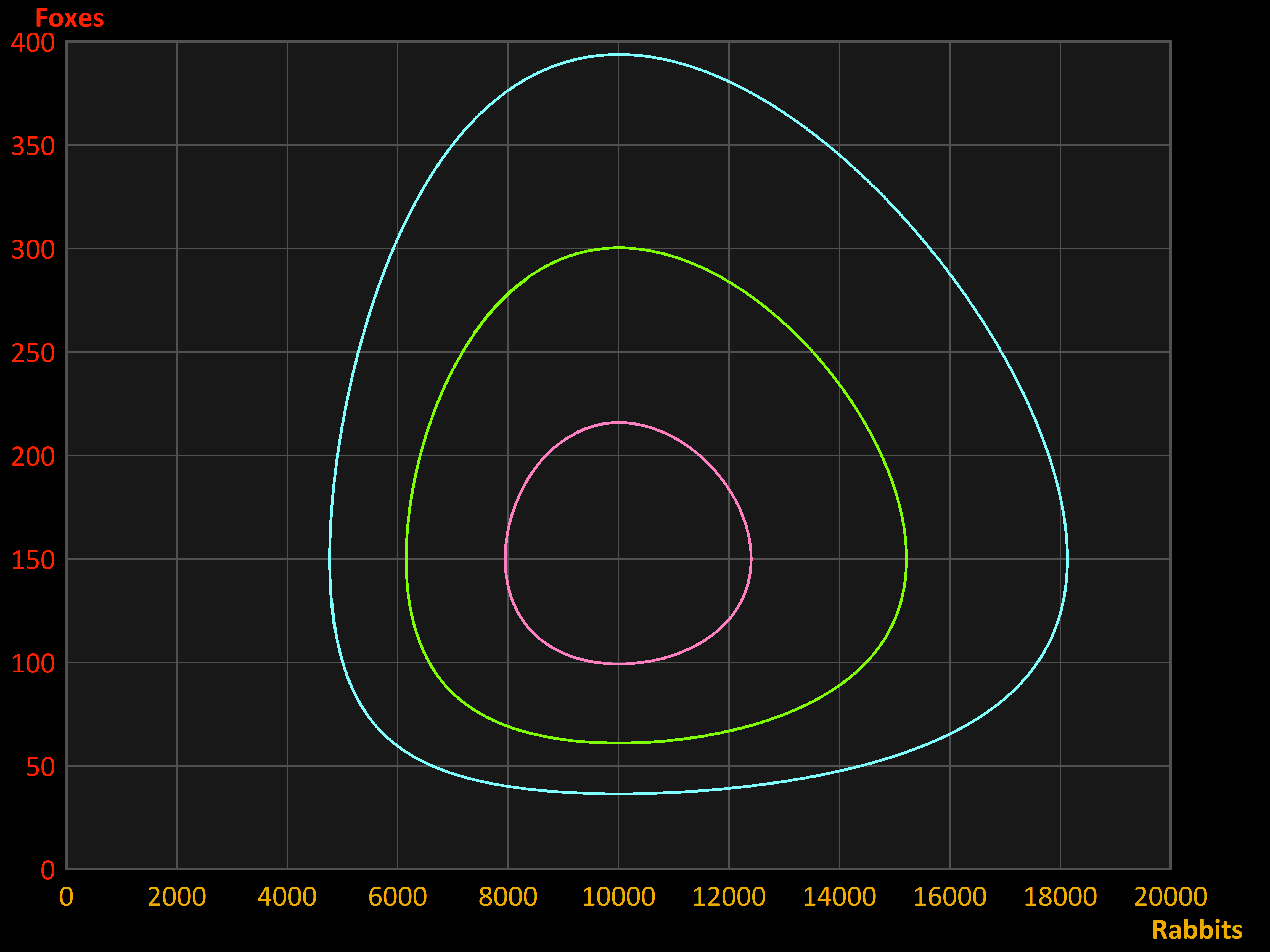
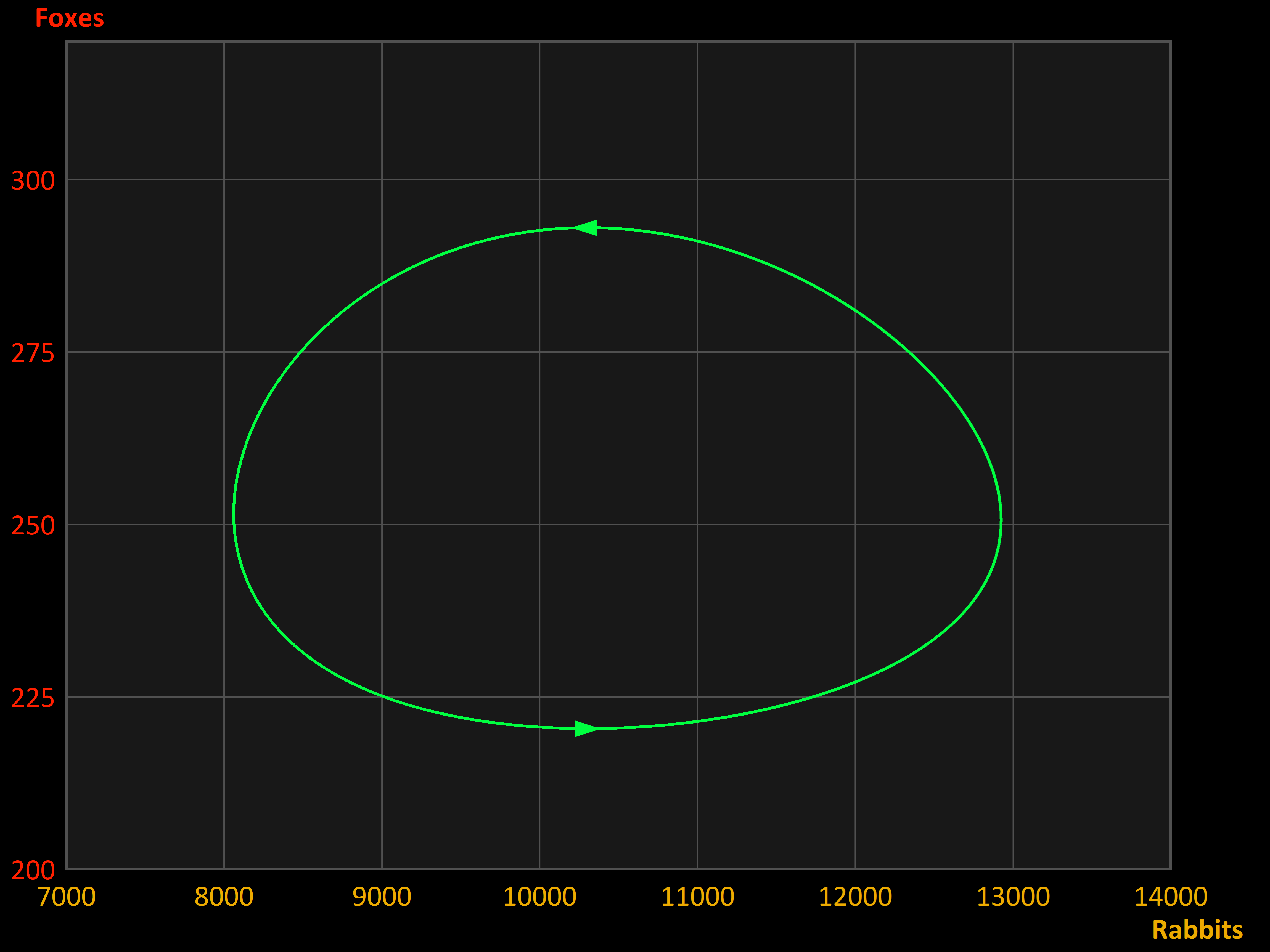
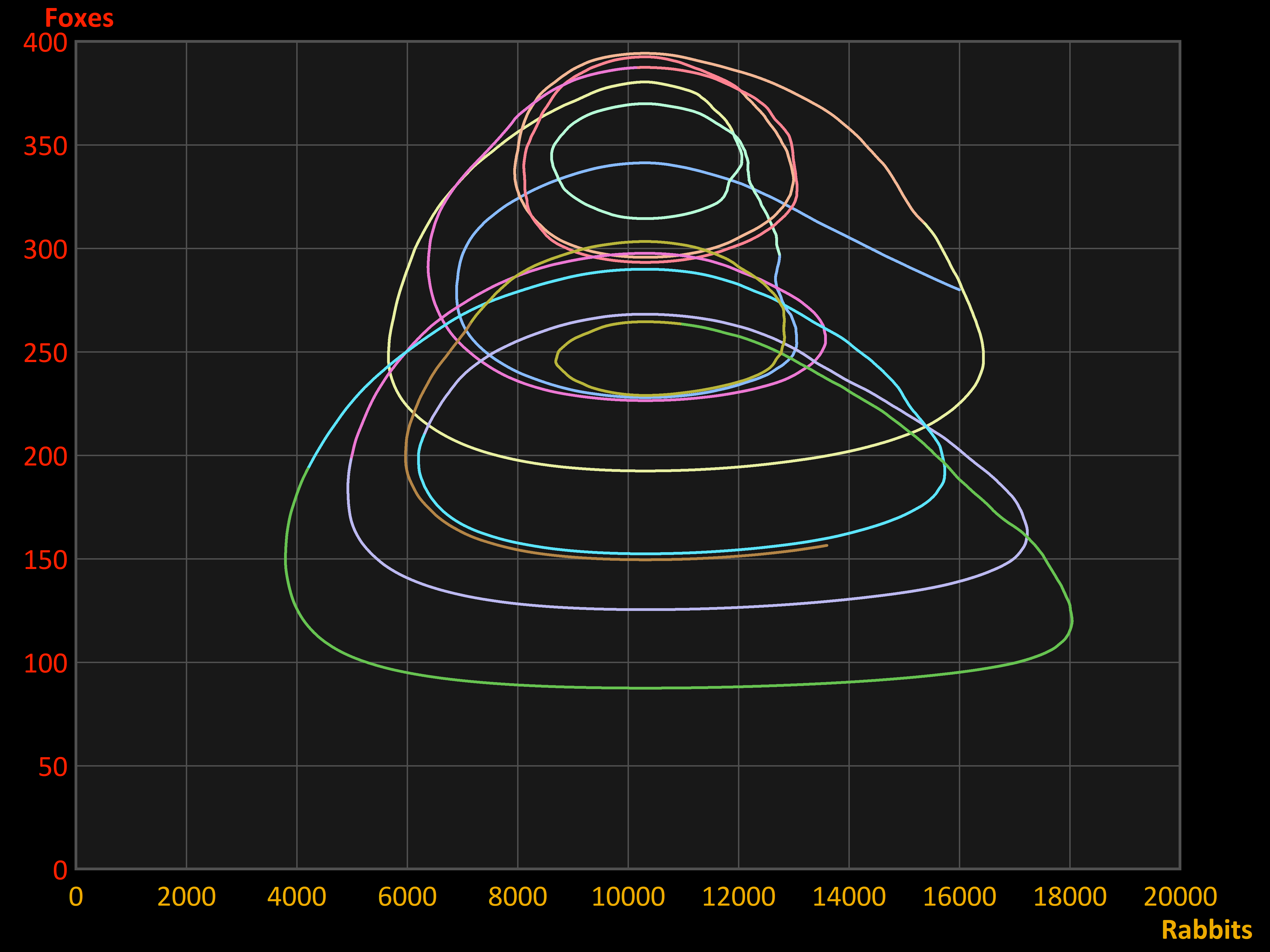
Development towards a limit cycle

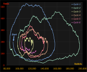
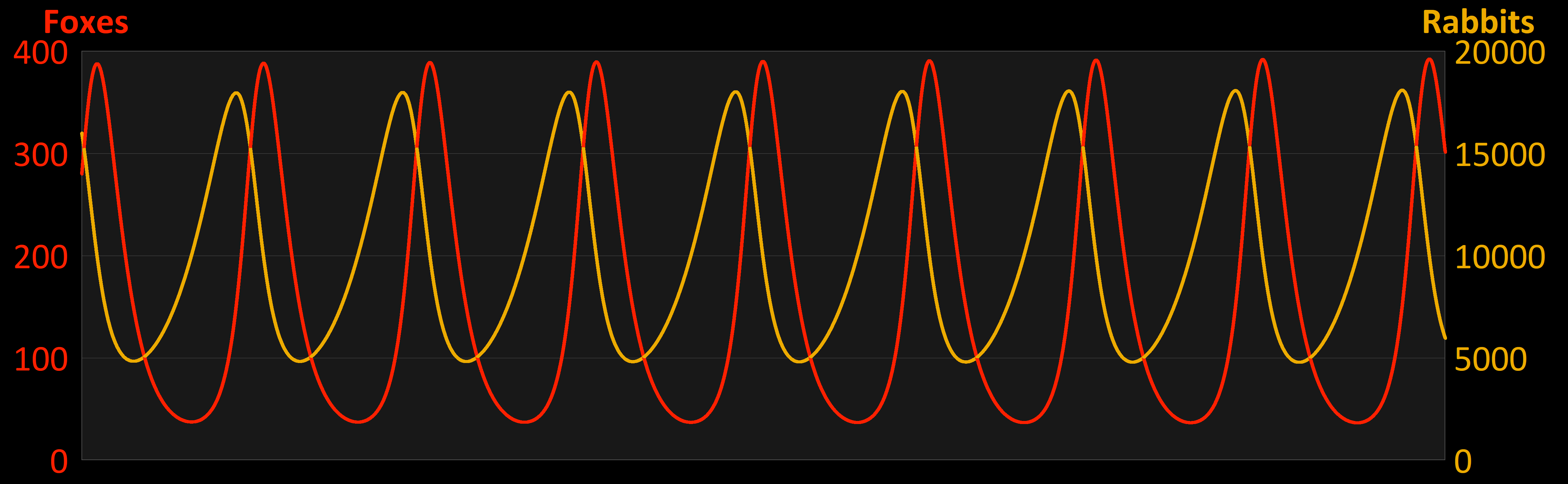
The result is, that the system reaches the limit cycle and then maintains this dynamic equilibrium. If no disturbance takes place, the system will indefinitely continue to go through this limit cycle, depicted in the upper left image below in green.

The size of the limit cycle can be influenced in the computer program by adapting values of certain parameters, for instance the catching skills of the foxes.

However, changing the number of foxes or rabbits at the start of the simulation (at
t = 0) does not have any influence on the limit cycle: whatever starting point in the phase diagram is chosen, the same limit cycle will always result. The same is true when - during the simulation - the animal numbers are suddenly changed in a rather crude way: through disasters. Several kinds of disasters can be started by a simple push on a button in the program.

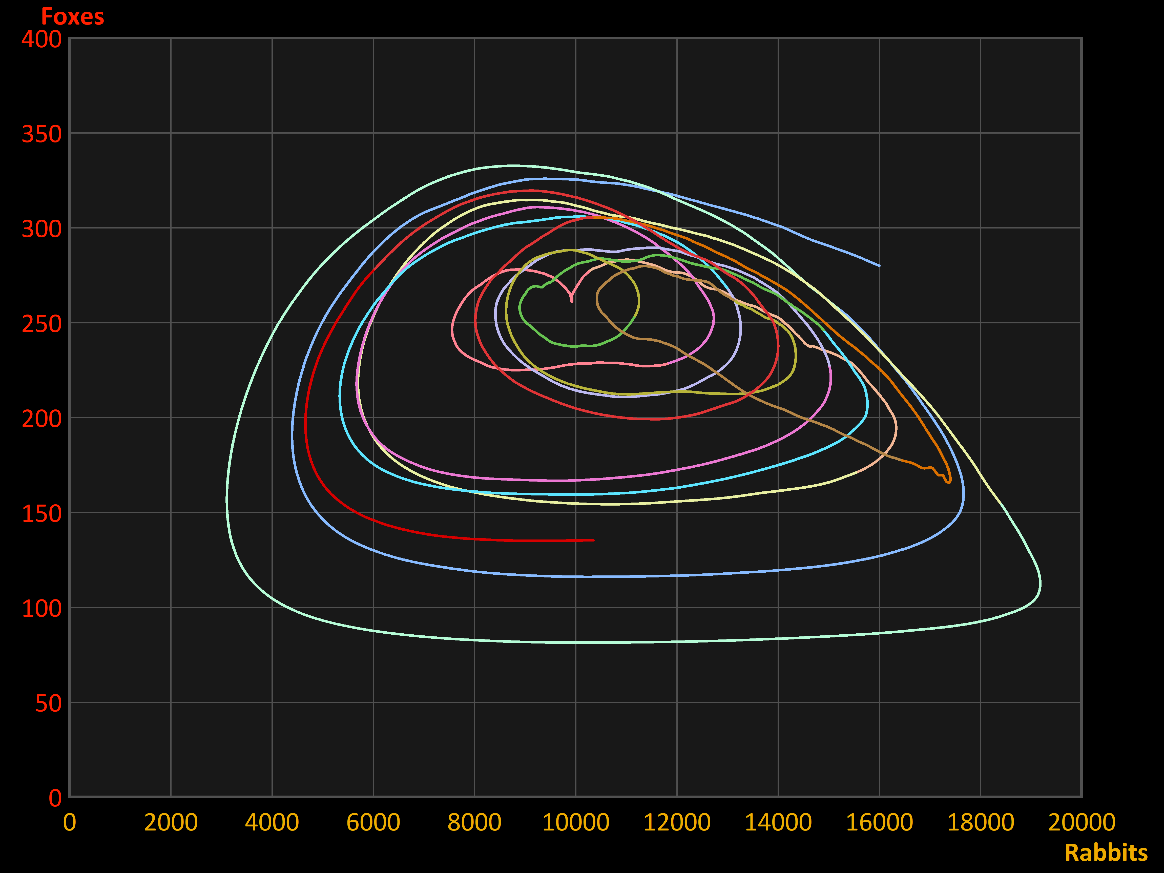
One of these disasters is an epidemic among the rabbits. The effect is shown in the upper right image, where the red arrow is the sudden result: the rabbits are more than halved. This brings the system pretty much out of its dynamic equilibrium. But, after a number of cycles, the original dynamic equilibrium is restored. (Mind the scales on the axes, which differ from the image on the left: the green-colored limit cycle is really the same.)

Dynamic equilibrium in a limit cycle

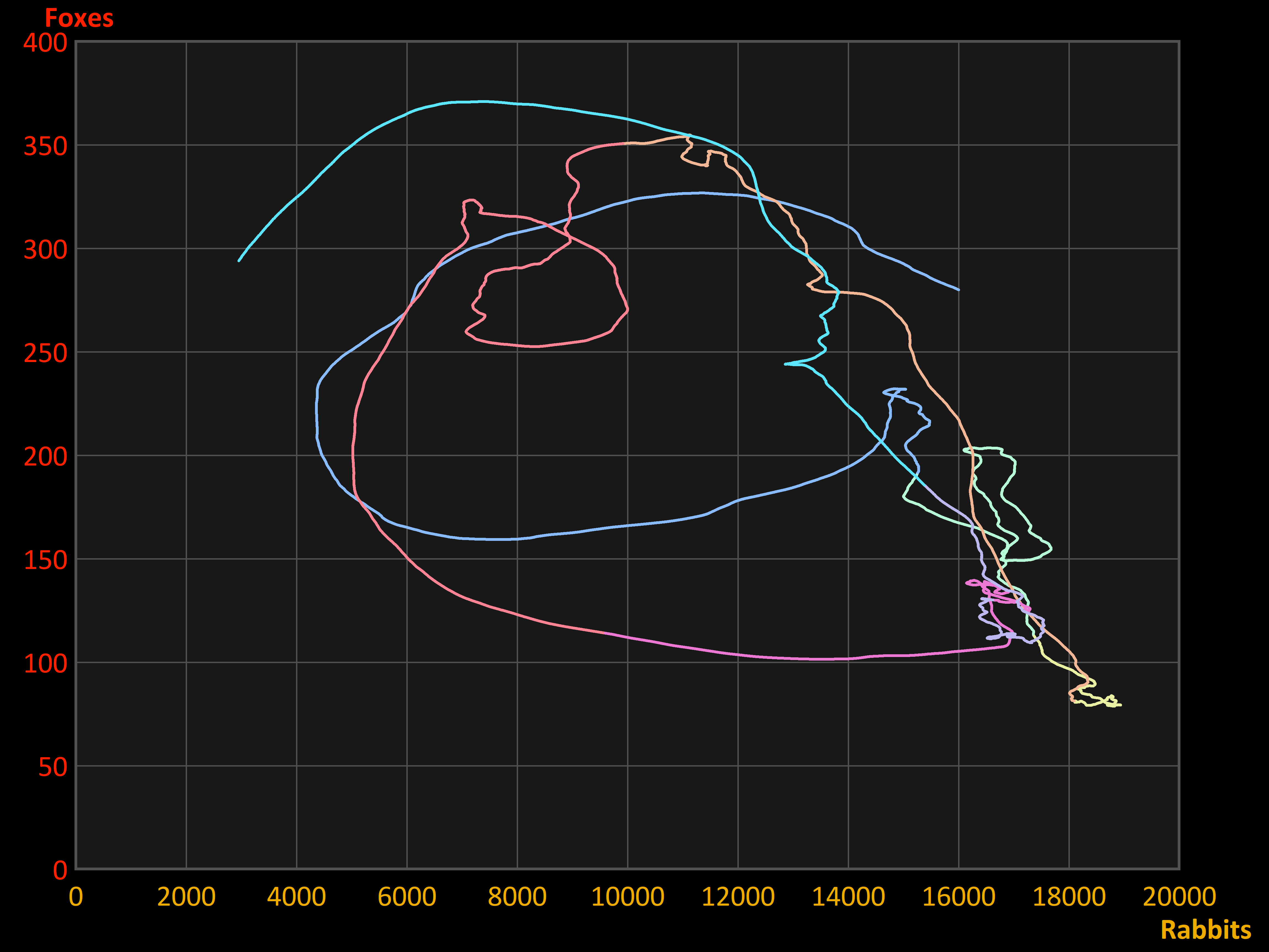
Disaster 2: forest fire.
The limit cyclew is reached again, this from inside out.

Disaster 1: rabbit epidemic.
After a while, the system reaches the limit cycle again.

Disaster 3: halving the biocapacity.
This is too much: this time the fox population is extinguished.

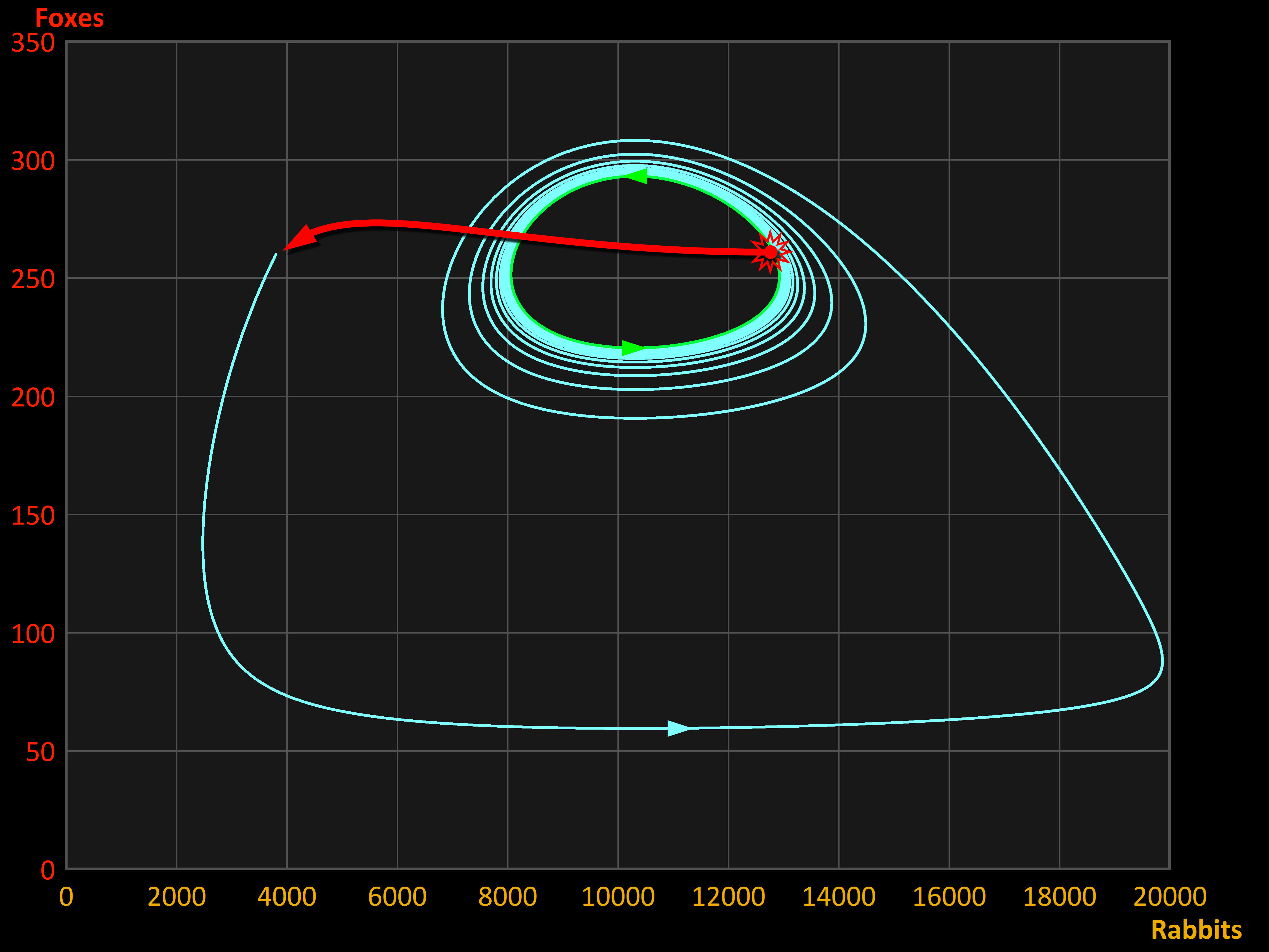
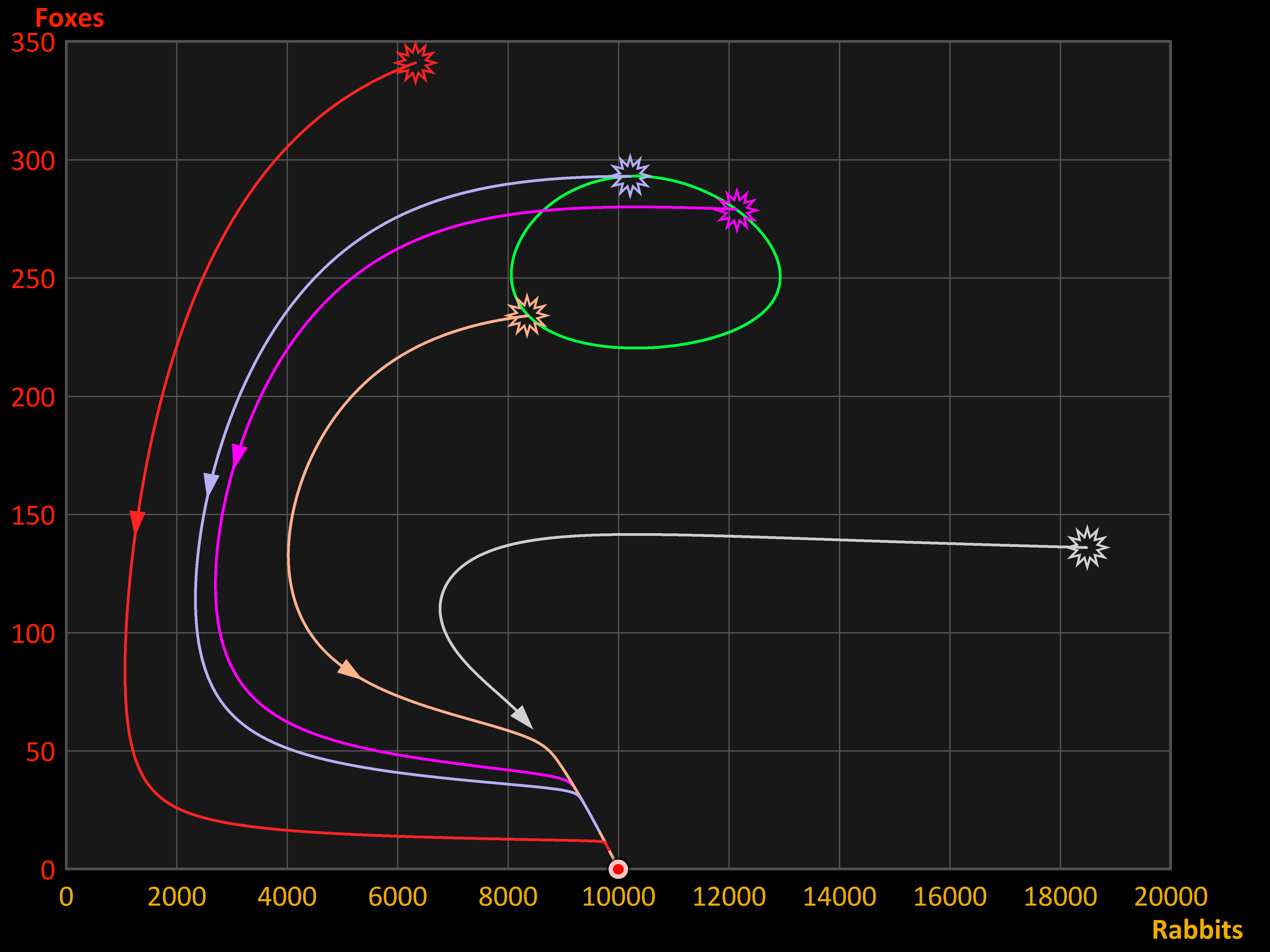
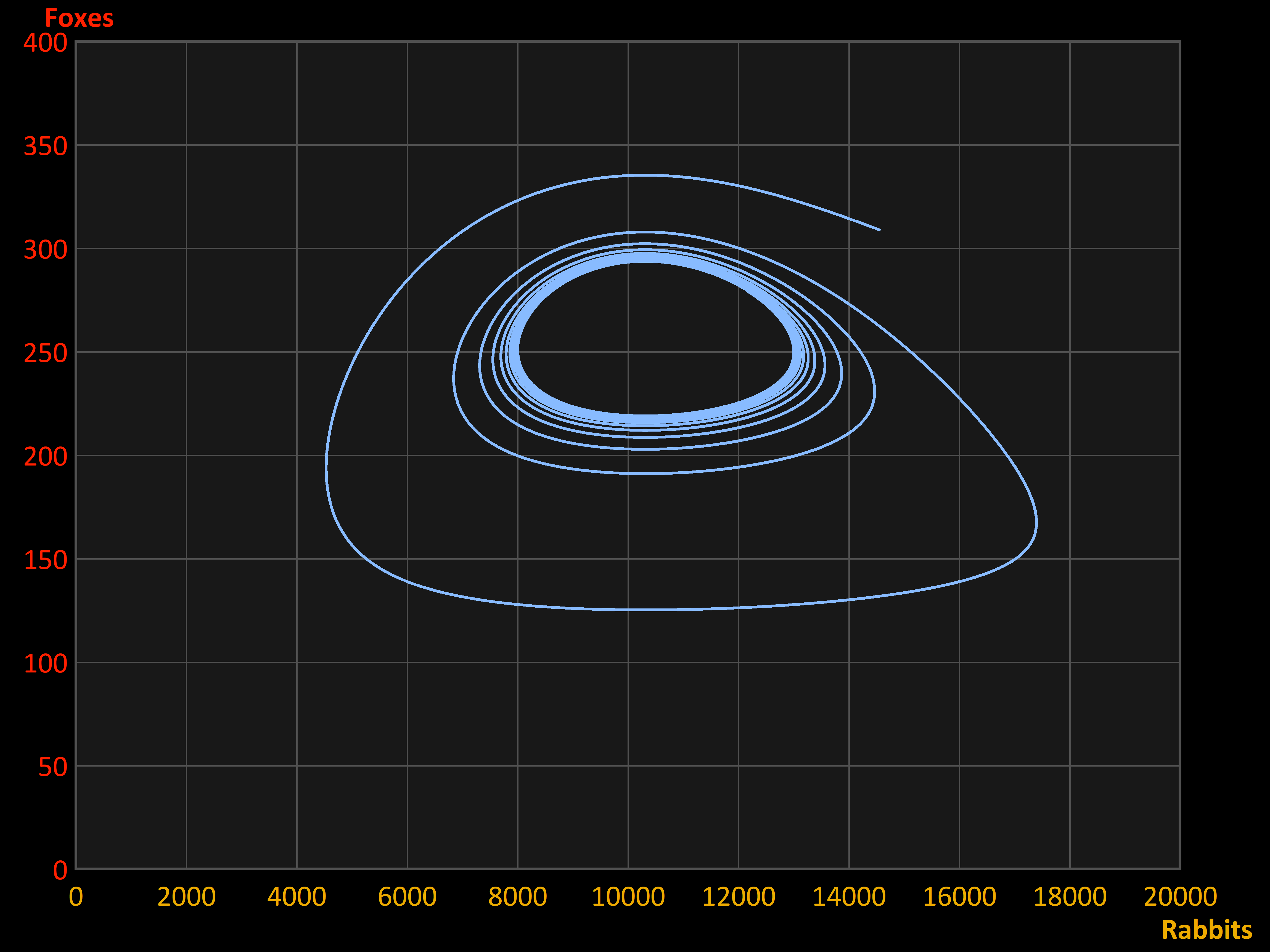
Disaster 2 also strikes heavily, when this time both the numbers of rabbits and foxes are lowered considerably in a split second. This is shown in the lower left image. This time, the disaster brings the state of the system within the limit cycle instead of outside. Nevertheless, again the original limit cycle is restored after a while.

But: certain disturbances of the system may end up catastrophically. This is the case when disaster 3 strikes. This time, one of the basic system parameters is hit, as the biocapacity halves. One might expect that some new dynamic equilibrium will be found. In some cases, when the biocapacity is damaged less, this will be the case. But decreasing the biocapacity too much will, as the lower right image illustrates, break the system and end up in the extinction of the foxes.

Of course, this is just a simulation, based on a model, i.e. on a simplified representation of reality. The conclusions from this model don't have any predictive power for the real world, right?

But perhaps they can serve as a warning. There is an important lesson to be learnt with respect to (un)sustainability. Damaging an ecosystem severely, even if only partially, may cause unpredictable catastrophes.


Randomness: Stochastic Models

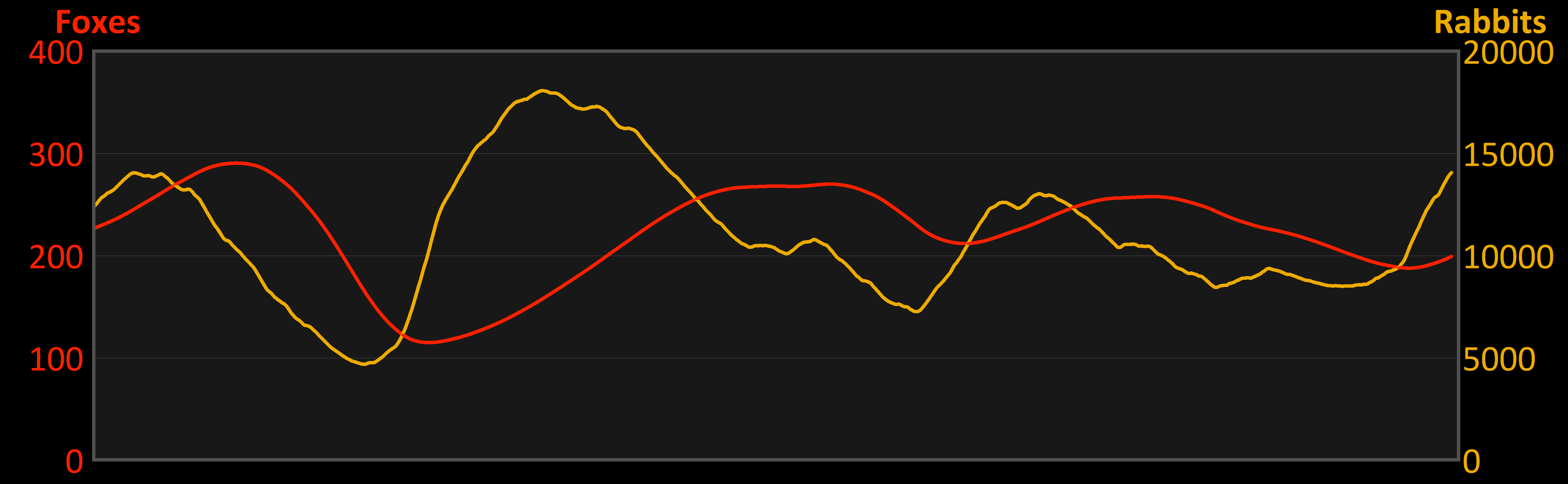
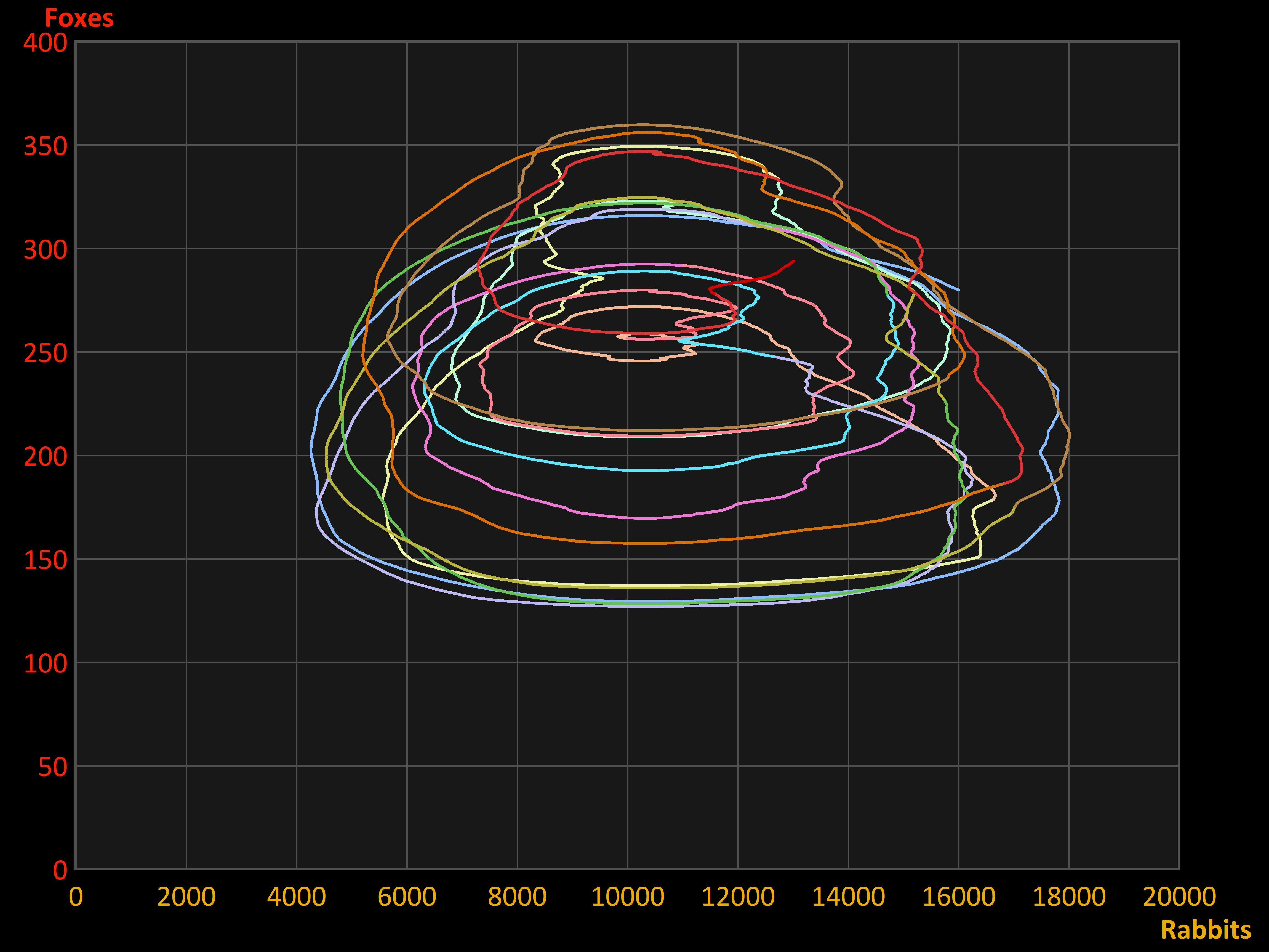
Speaking of 'unpredictable': Both models that wer descibed above have one weakness: they aren't unpredictable, as their outcomes will always be the same when the starting state is the same. There is no randomness.

The computer program, however, enables the user to introduce such randomness. This is true for both models: the Lotka-Volterra Model and the Logistic Model. On this page, randomness will only be shown in the Logistic Model; the reader is invited to experiment with it in the other model as well.

In order to create randomness, all basic parameters can be switched from constants to stochastic quantities, varying at random between certain boundaries. They don't jump up and down between those boundaries from moment to moment, but instead vary gradually - but unpredictably.

Time graph of the Logistic Model. Stochastic: only Rabbit Fertility

The user is able to select which parameters are switched to stochastic variables: one, several or all. In this mode, the resulting graphs are unique and will never be repeated.

In order to be able to discern the different cycles, the computer program automatically switches regularly to new colors. (The colors themselves have no meaning.)

Stochastic: Rabbit Fertility & Fox Hunger

The graphs produced in this stochastic mode will show patterns that - although unique - show characteristic types of shapes, as the examples show.

Stochastic: Fox Hunger

The fascinating question now is: does this kind of behaviour resemble any aspects of the real world?

Stochastic: Fox Mortality

This question will be answered first by comparing the Fox Rabbit Math Model with another computer program, based on a very different simulation principle: Fox Rabbot Field Model, described on the next page. This will be followed by a study of three different real-life cases.

Stochastic: all

< Previous page       Back to Top       Next page >