|
|
Chapter 1: The Machine that Knows the Truth
Unimaginable! What happened to me when I started to investigate something that seemed so simple.
How could I have known, that an investigation into a simple mechanical toy would lead me towards a whole range of new worlds. Weird worlds. Different. And yet in some way familiar.
I will show them to you, and you will be amazed. Just as amazed as I was when I saw them for the first time – and just as amazed as I really still am.
How it all began
As a matter of fact it started years ago, when I was a teenager. Every once in a while my father received some small gifts from one of his business partners. Usually he gave them to others. One time I got it, perhaps my father thought I would like it.
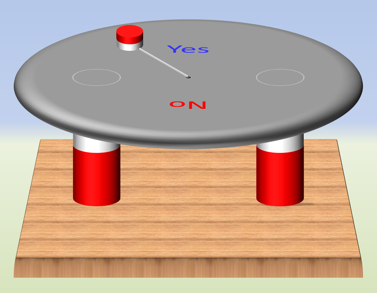
And I did, as it was a Yes-No-Machine. Indeed: a Yes-No-Machine. It was a simple piece of equipment, constructed on top of a small kind of table made out of plastic. In it, two tiny magnets were hidden. Both with their magnetic south poles on top. Or their north poles, I don’t know – I’m just guessing.
On top of this plastic table an arc was set up. Connected to the arc was a pendulum, which was able to swing freely. Attached to the bottom of this pendulum, there was another tiny magnet. This time with its south pole at the bottom – or perhaps its north pole, I was just guessing, remember? Anyway, in the opposite orientation compared to the two fixed magnets, causing it to be repelled by both of them.
Well, do take a look at the picture.
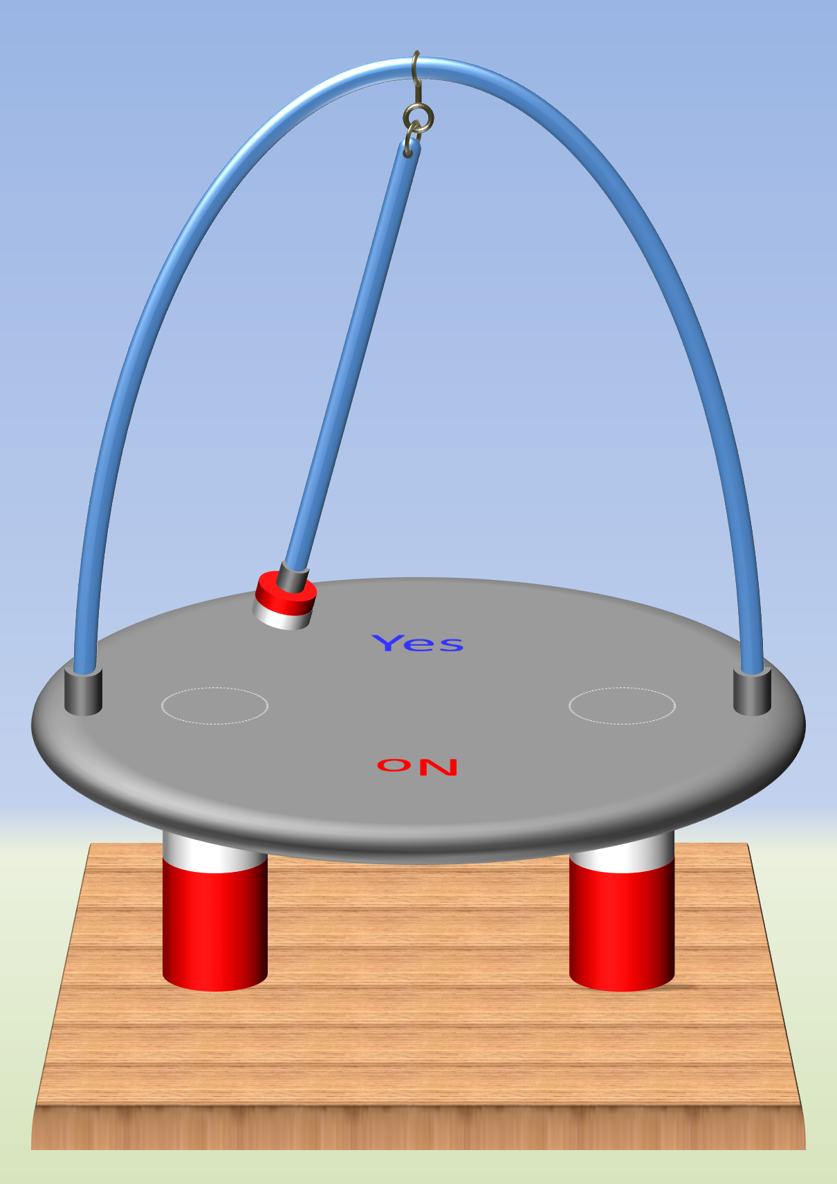
It was not exactly like in the image, I changed it a little bit. Actually the two fixed magnets were much thinner and they did not stick out at the bottom. Consequently there wasn’t any wooden board underneath, as it was not necessary at all. But if I had drawn it like that, you would not be able to see the two magnets, and perhaps some of you might not have fully understood it.
As the swinging magnet was repelled by the two fixed ones, the pendulum would never hang down vertically in a stable position. Two different stable positions were possible: in between the two fixed magnets, either hanging a little bit to the front or a little bit backwards. Exactly below those two positions, the manufacturer of the apparatus had painted the words ‘Yes’ and ‘No’. And – you probably guessed it – whenever you had a grave existential question, and you did not know to answer ‘Yes’ or ‘No’, you grasped your Yes-No-Machine, you gave a firm but not all too destructive push against the pendulum, you just waited for a quarter of an hour till the pendulum was hanging still – all right, rather a few seconds – and you had the answer!
Actually the machine was nothing more than a classy die. Or a two-sided coin that you toss with. But the Yes-No-Machine was special, as it knew the Truth and it was able to teach us wise lessons. Right?
The manufacturer will never have realized that this simple equipment would present a passage to mighty secrets. To other worlds! Weird and yet strangely familiar.
Years later, when I was programming
I too did not realize this, as years went by. Over the years in some way I must have lost the Yes-No-Machine, I can’t remember when or how. Pity!
I grew up from teen to adolescent and I started, 17 years of age, studying astronomy, which included a lot of physics. After a while, magnetic forces did not conceal many secrets from me, just like gravity or friction. Their mathematical formulas are easy, at least in classical physics, by the time you graduate. But the Yes-No-Machine had left my mind.
Then, the computer entered domestic life. It was still far from the present stuff, but there was one thing you could really do with it even then: write your own computer programs. For me, a new hobby was born. At that time the Yes-No-Machine came back into my mind.
‘Would it perhaps be possible to simulate a Yes-No-Machine on a computer?’ I spoke to myself. I often speak to myself. ‘If so, I would have my machine back, albeit virtually, behind the glass of my monitor!’
This was a nice challenge, and I went to work.
To start with, I inserted a minor simplification. In a real Yes-No-Machine the pendulum moves not only to the front and the back and to left and right, but necessarily also vertically. In other words, it is a three-dimensional motion. As such that is all right, as this can all be described in the mathematical formulas that you can teach to the computer.
But it makes calculations complex and hence slow. Please realize: in those years I was working with a computer that was thousands of times as slow as the one standing on my desk at present.
Calculation efficiency therefor was essential, and so I simplified the picture a little bit. I replaced the three-dimensional swinging motion by a horizontal sliding motion, where the role of gravity, striving to draw the pendulum downwards and hence towards the center, was adopted by a pulling spring, or an elastic if you prefer, also pulling the moving magnet towards the center. You already noticed the new image, I gather.
The rest was not that hard. The kind of computer program that is involved here is a ‘simulation program’, i.e. a simulation of reality. In order to do this, you select an arbitrary starting position for the moving magnet. For this position you calculate – actually you make the computer calculate – the forces that act upon it, and there are three of them: two magnetic, and one elastic force. As soon as the magnet starts moving, a fourth one enters the stage: friction.
You add up all of those forces and you divide the result, just as Sir Isaac Newton taught us in 1687, by the mass of the magnet: this is how you get the acceleration of the moving object. In order to increase the calculation speed, of course I chose a mass of 1, so the division can be left out altogether.
From the acceleration you calculate the speed the magnet acquires. From its speed you next calculate the change in position, all during a tiny piece of time, e.g. a hundredth of a second. From the positional change you calculate the new position, and then it starts all over: again you add all forces, etcetera. This is repeated many times, e.g. a million times, and the entire motion appears before your eyes – that is, if you keep them pointed at the monitor.
This neat trick is applied in all places! Like, when you are watching the weather forecast for tomorrow on TV, the weather station did exactly the same: it put all weather data of the present in a supercomputer, let the simulation roll for a while, and voilà: tomorrow’s weather. If you’re lucky, that is, cause the weather is highly complicated, far more complicated than the math the meteorologists fed to the computer. The weather is a complex system.
With my own private simulation, after a few days of crafting and programming I succeeded in getting nice images on my screen. I’ll show you one of them. It is the motion of the magnet, as seen from above.
At the right, below, the sliding magnet has its starting position, which I chose at random (by clicking the mouse somewhere). When I released it (virtually, digitally) it started to slide to left and behind, raced through the center, was disturbed in its motion by the repelling fixed magnets, and came to a rest after some ten wild loops thanks to friction. In a ‘No’ position. At least I think, as the word is not visible in the image, 'cause I forgot to add it.
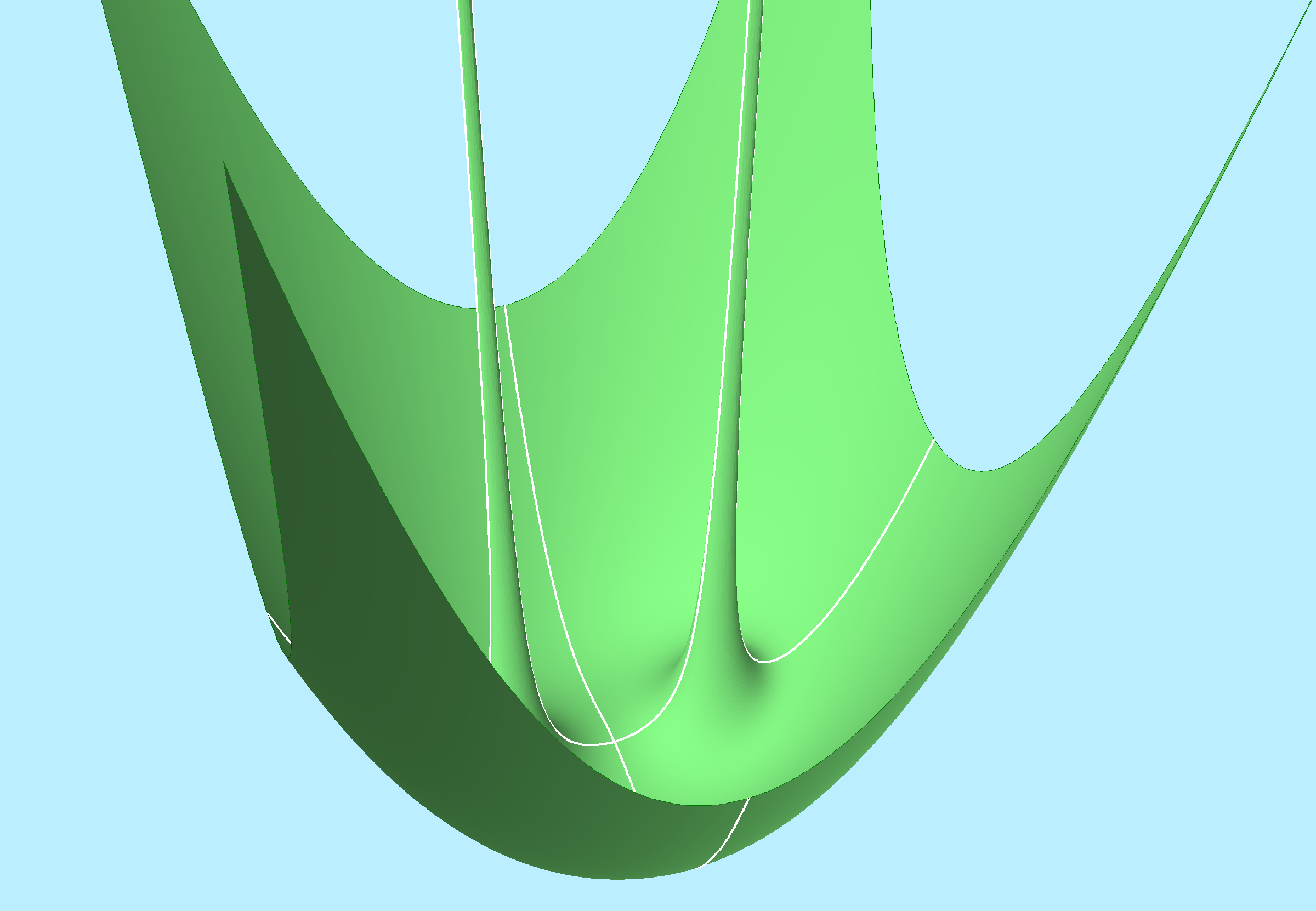
This motion can be pictured in a very nice way, when you imagine the table on which the magnet slides as a kind of hilly landscape. Repelling magnets feel as if you have to cycle uphill when you approach them, and it is possible to draw those hills in a picture.
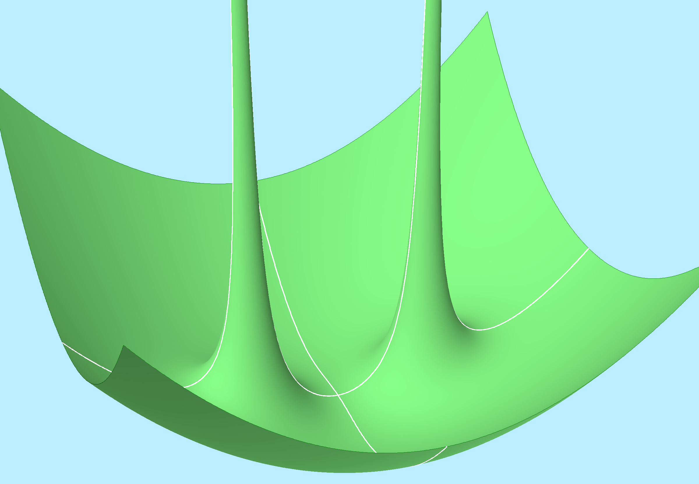
The landscape as a whole, neglecting the two hills caused by the fixed magnets, has the shape of a bowl. This is due to the elastic force, attracting the moving magnet towards the center, as if gliding into a soup bowl.
By the way: for the physicists among you – a small family meeting, just for a few seconds, sorry – this landscape of course is the potential field, right? (I would like to add briefly in small print that I simplified the system in some more ways than just the replacement of gravity by the elastic force of a spring. E.g. I pretended the magnets to be simple monopoles, I hope you don’t mind...)
Without the two magnets the center of the bowl would naturally have been the lowest point. But thanks to the presence of the two (infinitely) high peaks this central point is lifted a little bit, and so two other places have become the lowest spots in the landscape, i.e. the places where the moving magnet may come to a halt. Those are the spots where I forgot to paint the words ‘Yes’ and ‘No’, you see?
‘Nice,’ you may think. ‘But that is not really an amazing new world: just a bowl and two mountains. How would that be sensational?’
Actually, it isn’t yet. But then I discovered something else.
Chapter 2: The land of Yes and No
My goal was reached: I was able to study the orbits of the moving magnet. I could even answer difficult life questions with ‘Yes’ or ‘No’, using my virtual machine.
Satisfied, I leant back in my chair. But not for long, because: when you have such a result in your hands, you start thinking. At least, I do. Like: would it be possible to select the starting position of the magnet in such a way that you know on beforehand whether you will get ‘Yes’ or ‘No’? To put it differently: can you cheat? Or, more generally: which starting points will end in ‘Yes’, and which in ‘No’?
Of course, there was only one way to find out. You simply test a whole lot of starting points, and each time you see what you get. Better still: test every starting point!
This called for a new job for the programmer in me. The program had to walk systematically along all pixels of the screen. Point after point, row after row, every pixel of the screen from top left to bottom right. Starting from each point, the program had to perform the complete simulation, in order to investigate if it ended in ‘Yes’ or ‘No’. The exact orbit of the moving magnet now was not relevant anymore, I didn’t need to see it: I was only interested in the final result. I could create a nice picture of it: a sort of two-color map. Every point on the map delivering a ‘Yes’ received a bright color, every ‘No’-producing point a dark one.
After another couple of days of programming – fantastic hobby that is – I had convinced the program to do as I wished. Excited, I waited for the result. Slowly, very slowly – I had a fairly good computer, for those days – but… those days, right? – the map came into being. While it grew, my amazement grew too. I was stunned.
The result was beautiful! This was truly art, or rather: Art. Please look at the picture.
Certain areas appeared to behave neat and tidy. There, the ‘Yes’ and ‘No’ regions are lying next to each other in broad lanes. But other areas are absolutely crazy. Here, the ‘Yes’s and ‘No’s are fully clutched through each other. Completely chaotic, at first sight. But at second sight with some kind of structure. Fascinating!
Of course this required further study. What would appear before my eyes when I zoomed in on such a complex region?
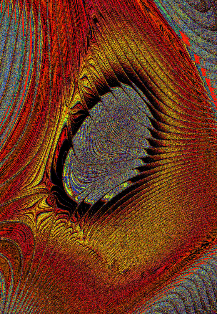
There was one way to find out: expand the computer program with a module ‘zoom in’. This gave me a couple of days of thrilling new programming work, until I was able to select an arbitrary rectangle with the mouse, after which the computer enlarged it to the entire screen. I’ll show you one of the results. It is the result of a repeated magnification with finally a factor of ca. 34,000, zooming in on such an apparently chaotic area.
This and comparable examples made clear that I was able to zoom in truly as far as I wished. Over and over again I discovered fascinating new views, combining orderly next to seemingly chaotic regions. At a certain moment I had reached a magnification of a hundred billion (1011) times, and again chaos appeared to contain order. If I wanted, I could repeat this process to infinity! That is, until my dying day, hopefully due to old age.
This implied that I was not dealing with a chaotic but with a complex structure. With ‘complex' in its mathematical meaning of the word. In other words: the image is a fractal.
I don’t know if you are familiar with the term ‘fractal’. It relates to images with a certain mathematical background. The first fractals were designed around 1975 by Benoît Mandelbrot and are named after him. If you google on ‘Mandelbrot’, you will get all sorts of results.
Indeed my computer simulation of the Yes No Machine looks very similar to the construction of a Mandelbrot. In both cases the process is recursive, i.e. repeats itself a great many times, applying the results of every process loop as the starting point of the next one. In my case this is the repeated calculation of forces, accelerations, velocities and transpositions, with which I calculate the track of the moving magnet.
While experimenting, I thought of something else. Wouldn’t it be nice to use, instead of the yes-or-no-answer, the decision time as a measure for a map? If, for each starting position, I would record the time it took to reach a ‘yes’ or a ‘no’, and then interpret that time as a color for that starting position: what would come out of that?
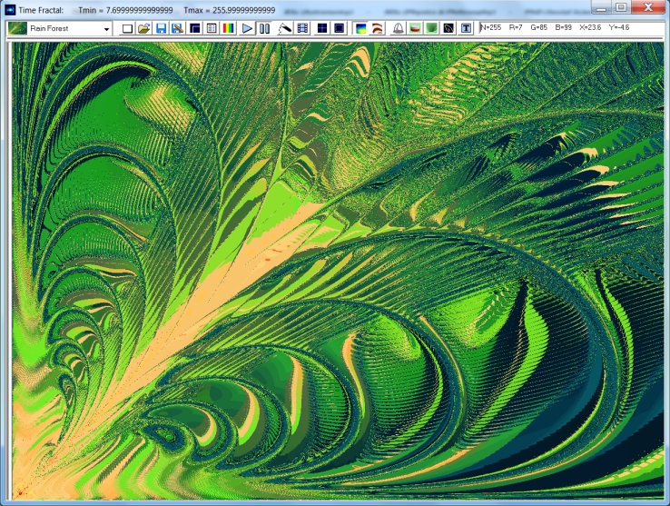
Well, in the next few programming days I designed a color code. Black represents the fastest decisions; blue stands for the ones needing a little bit more time; and so on. The result below can be compared with the first image in this chapter: it covers the same region. Isn’t it beautiful?
My first ‘world’ was born. Fascinated, I entered and explored this world. Once I zoomed in on a kind of ‘island’ visible on the entire world map, on the right, somewhat below the equator. This region is shown below, twice: first as a time chart, next as an endpoint map. If you look carefully at the world map above, you will find the island, I guess.
On the world map you will find two isolated tiny isles, both on the equator. I named them the East Pole and the West Pole. They are exactly located at the positions of the two fixed magnets.
Of course it is exciting to study these poles carefully. I show you the East Pole.

Do you realize what a magnification of a hundred billion times means?
If I would print the ‘world map’ with a width of a meter, the photo shown below would be smaller than the size of an atom.
The image is shown in both styles: time chart and endpoint map.
Chapter 3: The colors behind the rainbow
Again, years passed. Technology moved forward, and so – not very long ago – I possessed a computer with, compared to the one I originally simulated the Yes-No-Machine on, possessed fantastic capabilities. Especially concerning speed.
On a nice day I decided to return to my former adventure. And for a reason, because: where my earlier, archaic computer sometimes needed a day and a night for the production of one image, the same could now be done in maybe five minutes. This discovery was to me the beginning of a great adventure, in the course of which I was to travel across many exotic universes.
The cause was this: I suddenly realized that the first world I had discovered did not need to be the only one! This world was based on one particular physical stage play, in which two fixed and one moving magnet star together to determine the laws of nature and hence the cosmic structure of its universe.
What would I get to see if I chose a different theatre? As an example, I could fantasize that the force drawing the magnet towards the center would be stronger, by not being proportional to its extension as usual (as expressed in Hooke’s Law), but with its square. The bowl in the landscape then becomes much steeper, as the force is stronger.
While renewing my explorations, I could just as well add other options to my virtual laboratory. Entirely new forces. New objects, obstacles, frictions, attractions, repulsions, rotations, and so on. To my mind, endless variations appeared. Would I be able to get them on my computer screen?
You will understand: many brave programming days were ahead. But not just to explore new worlds – where no man had gone before. Because, you know – if I did not invent the shapes and the structures of those worlds, I did have the ability to influence their color patterns. In the full-color time charts I had even more freedom than in the two-colored endpoint maps.
For the world hidden behind the Yes-No-Machine I had designed a simple color code. As I told you: black stands for the shortest decision times. Blue for longer ones, and so on through green until yellow for the longest times. But of course much more was possible!
The first thing I needed to do was to design a program module that allowed me to freely design color patterns. You see this module here: the image shows the simple color pattern of the Yes-No-Machine.
In the new world I explored, the one with the stronger attracting force, I discovered a truly fairy-like landscape. I will show it all in the next chapter. In that landscape, many more colors appear than the usual seven rainbow colors. I designed the following exotic color scheme.
And so, after a while, I had the program running again to paint me a world that went beyond my imagination.

Chapter 6: Those physics, is that magic?
It's amazing! It seems like magic: how, just by replacing a few lines in a computer program, you can discover a completely different world.
Discover? Or should I say: create?
Like: ‘In the beginning God created the heaven and the earth. And in the third millennium I created some more.’
No. No, no. I don’t think that is right. The only thing I do is, typing in hundreds of variations of the good old physics formulas – for gravity, for frictions and magnetic forces, etc. – and next wait with a quickening pulse to see what the program will set on my desktop.
In 95 out of 100 cases this is nothing but rubbish, and I seek further.
But it’s a fact: given the formulas, the world is fixed. If someone else would fill in the same formulas in a suitable computer program (which he or she would have to write first, all right), then that program will show the same world.
All right: I choose the color combination, I admit. But the shapes, the structures, the consistencies, in short: the laws of nature of the associated world, they are determined by the formulas.
So my opinion is: I am not a creator of worlds. I am an explorer. And after I explored these worlds, I am your guide and I lead you around.
In this chapter I will offer you the chance to nose around in a few plainly bizarre worlds without explaining a lot to you.

And eh, maybe you yourself are a programmer, or a physicist or whatever, and you think: ‘You know – I would like to see a couple of those programming lines!’ Well, all right. Below I will show you a few lines. If you don’t like it: you can simply skip them. So don’t blame me.
For the experts among you: the programming language is Delphi, you will recognize it. Version 7.0, in my case.
Do you remember how I explained the notion of a ‘simulation’, in chapter 1? I mentioned there the forces that influence e.g. the motion of a magnet within the Yes-No-Machine.
What I did not mention then is that actually you have to distinguish two kinds of forces: one in the x-dimension (horizontally), and one in the y-dimension (vertically). That is why, in the computer code I showed you, each case makes use of both Fx and Fy.
(In physics, ‘F’ is short for ‘Force’, so there you are.)
In fact, in each and every case it is only those two lines, the ones for Fx and for Fy, that make the difference. The black colored lines that often precede them are just subordinate clauses that make the calculations clear and efficient.
And so, it is really true: replace two lines of programming code, or adapt a couple of characters or numbers within them slightly, and you will discover a brand new world. That always was there, of course. We only did not know that yet.
Magic? No, reality! That may be the reason why, even if a world is totally new and strange to you, it may offer a vague feeling of familiarity. As if you knew it already, somewhere deep inside.
The wonderful thing is: in real physics, that of OOU (Our Own Universe), it is exactly the same. Here too, just a small number of basic formulas suffice, together with a couple of universal constants of nature, to determine the universal structure. One such constant is the speed of light: 299792458 meters per second.
It is highly surprising, that OOU is so simple in its physical basis, and at the same time it is so incredibly complex in its realization of it in our biological and human existence. It seems like magic… but it is not. It is reality.
Equally surprising is the fact that you can copy this OOU trick with the aid of a simple computer program, discovering other complex worlds thanks to two programming lines. Beautiful, isn’t it?